💻 usethe.computer

Blood From a Stone

2026-04-08

This post originally ran on Collide, a social network for the oil and gas industry, as part of a technical writing contest; it appears here with minor edits. My goal here was to give non-programmers a peek into some of the fun we get up to when reverse engineering data formats (and sometimes software).

The poll was a landslide - the people insisted upon the reverse engineering war stories. There was, however, one problem.

SOCRATES: …Thamus replied: O most ingenious Theuth, the parent or inventor of an art is not always the best judge of the utility or inutility of his own inventions to the users of them. And in this instance, you who are the father of letters, from a paternal love of your own children have been led to attribute to them a quality which they cannot have; for this discovery of yours will create forgetfulness in the learners’ souls, because they will not use their memories; they will trust to the external written characters and not remember of themselves…
PHAEDRUS: Yes, Socrates, you can easily invent tales of Egypt, or of any other country.
– Plato, Phaedrus

I have always been drawn to programming because of my very limited memory. Having worked out a method for accomplishing a goal, I prefer to write this method down in such a way that it may be forever after executed by machine. Having done this, I promptly and permanently forget the details.

The events I hope to recount took place in 2023 and produced, in total, an open-source library and a few pages of indecipherable working notes. Since I have little memory of the path by which I arrived at these artifacts, I’ll be writing this narrative quite authentically: I’ll also be (re-)working it out as I go along; reverse-engineering my own reverse-engineering, Menard and Quixote both.

At the time I was working with a handful of clients who, in the same way these things always seem to converge, all intended in one way or another to re-interpret landing zones from public well records. This meant having geologists interpret formation tops and generate gridded structure maps for the potential targets, and then threading well trajectories from public deviation surveys through these in XYZ space. Which layer of the cake does the worm spend the most time traversing? A simple enough math problem, if you’ve got the numbers to work from.

Numbers enough we had, but not in the most useful form: geologists used tools like Petra or Kingdom to krige formation tops into the spaces between their well logs. These tools store their data in proprietary and opaque data formats; to extract gridded values required manual interaction to export an “XYZ file” or some other text-based format. It was a frustrating state of affairs to have a fully automated well-landing pipeline ready to run at “entire US” scale but bottlenecked on manual data exports every time a formation tops grid was created or revised. Was there a way to extract the relevant x, y, z coordinates from Petra .grd files without the Petra application or human intervention? You already know I wouldn’t ask the question if the answer wasn’t in the affirmative.

Reverse engineering carries a certain mystique, alongside nebulous notions of “hacking” and other dark digital arts. The truth is that all of us programmers are reverse engineers at times: “what was this guy thinking when he built this?” (usually “this guy” is in the first person). Broadly, reverse engineering in software involves making sense of either the operation of a program or the representation of data, usually without access to key information (that said, all too often making sense of a program even from source code is a reverse engineering exercise). The two are intertwined (program writes data is read by program) and the skills involved overlap considerably: familiarity with low-level details of computer architecture, experience enough to recognize common patterns, relentless pragmatism, empirical mindset, sub-clinical tendency to pareidolia. I am told that large language models can now supply many of these traits. In any case, it’s one of the lesser-known but more enjoyable (for me!) services I offer.

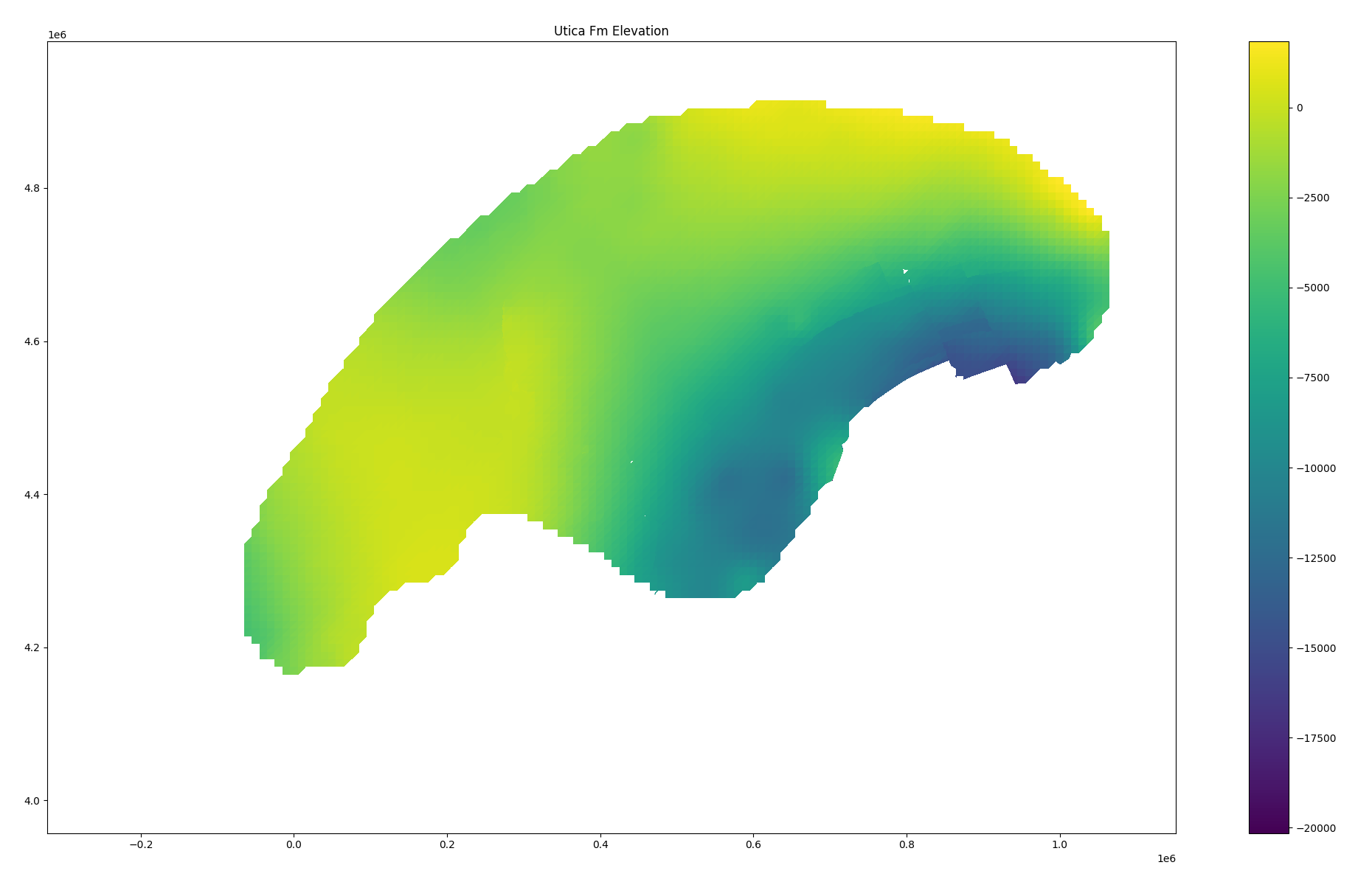
Now that the scene is set, here’s the part where I start lying. Tracing back through e-mail and personal wiki notes, it seems the investigation began with a Wolfcamp A grid shared by a client. We knew it had a “.grd” file extension and that was about all. I don’t have that file any more and couldn’t share it if I wanted to, so any examples I show henceforth will be taken from the West Virginia Geological and Economic Survey Utica Shale Play Book. This public data set (you’re looking for the “Supplemental Petra® File for Utica Shale Play Structure Contours and Isopachs”) contains structure and isopach maps for the formations of the Utica play across a few states. (Despite the real story mostly being about structure maps, we’ll be mostly looking at the isopachs today, because they reflect the simpler data format I worked out first; most of the structure maps are triangulated - more on that in a bit.)

Shame on us, for all we have done
And all we ever were, just zeros and ones
– Nine Inch Nails, Zero Sum

You’ve perhaps heard that computers use binary numbers to store data: it’s all just zeros and ones. This is, of course, true but in itself a useless factoid. The devil is, as they say, in the details (I have always felt there was a certain Faustian element to the art of programming!) but this article grows long before the first screenshot is placed. In short: there are a variety of conventions for encoding numbers, letters, images, and so forth into sequences of numbers, represented in the computer’s various “memories” in base two as patterns of “on” and “off”. Much of the data we work with is textual in nature and for this reason many of the file formats we encounter are “text files”; their contents are numbers which represent letters (graphemes? “code points”? hard question!) according to one standard or another (historically, ASCII with a growing tendency to various Unicode representations e.g. UTF-8).

Text is universal (just ask an LLM!); we can surely represent the third prime number as “five” or “5” or even “the third prime number”. Sadly, this doesn’t scale; even in ASCII (we can save some space if we assume incorrectly that everyone uses the Latin alphabet without töö máñÿ àçćëntş) we spend 13 bytes (= 104 binary digits) to represent (with commas) the number 2,034,799,123; represented “natively” as a binary number we can pack it into 4 bytes (= 32 binary digits). The situation only gets worse when we attempt to represent real numbers with fractional components and so forth. For this reason, and because it is in a sense “easier” for the computer and the programmer, we often reach for “binary” file formats for large quantitative data sets. This term only means that the data in the file isn’t intended to be interpreted directly as human-readable text via a standard encoding like ASCII or UTF-8.

All of this to say: if you open a Petra grid file in a text editor (like Notepad, or Vim, or Visual Studio Code) you’ll see “gibberish” for the most part:

A few tantalizing printable characters can be seen (strong evidence that there’s metadata embedded in the file as strings of ASCII text), but for the most part we see my editor’s representation of unprintable characters (that is, numbers which don’t map to letters, digits, punctuation, or symbols in the ASCII encoding it’s trying to apply to the file). We’ll need to reach for a tool better suited for analyzing binary file formats: a hex editor. Hexadecimal: another “hacker” term laden with mystique; visions of black cats and Salem graveyards at midnight. As always, there’s no magic, just the observation that base two and base sixteen have a nice relationship: one byte (eight bits, or base two digits) exactly maps onto two hexadecimal (base sixteen) digits. We extend the usual 0–9 digits with the “digits” A–F to represent ten through fifteen; place value works just as it does when we write numbers in everyday base ten. So, FF (base sixteen / hex) = 255 (base ten / decimal) = 11111111 (base two / binary); a byte of “all ones”. A hex editor lets us look at an entire file byte by byte as hexadecimal numbers. Good ones will also display ASCII or Unicode interpretation side-by-side with it, let us search for patterns, try interpreting sequences of bytes into different formats, and provide other contrivances to make the reverse engineers’ life easier.

I’m certain that in 2023 I would have done this work on Windows using the freeware HxD editor, but today we’ll be using my current “daily driver”, the open-source ImHex editor. It’s cross platform and will even run in your browser. Let’s take a look at an example from the Utica data set, UTICA_ISOPACH.GRD. (If you downloaded the dataset, you might enjoy loading it in the “Web Build” of ImHex, in your browser, and playing with it a bit.)

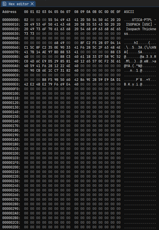
You can see the hexadecimal representation of each byte in the file on the left, with an “ASCII” column on the right to help us spot any embedded plain ASCII text. (As noted before in a text editor, the file name and description appear early in the file.) We see some numbers and lot of zeros.

This is not surprising. We haven’t the space here to get into why, exactly, but many binary format designs are primarily driven by ease of reading or writing them to or from data structures in memory of a running application. We often find a “header” containing some metadata at the start. This often begins with a “magic number” or “magic string” identifying the file format (pop quiz: if you open a file in notepad and see “PK” followed by gibberish, what is it? how about “MZ”?), followed by some human-readable text describing the file, followed by some important metadata required to parse the remainder of the file. What kind of important metadata? Data types, record sizes, array lengths and layouts: things the program needs to know before reading the “real” data.

Show me your flowcharts and conceal your tables, and I shall continue to be mystified. Show me your tables, and I won’t usually need your flowcharts; they’ll be obvious.
– Fred Brooks, The Mythical Man-Month

The .grd format is for data grids; these are two-dimensional arrays of some attribute (“z”) value over cells in x, y space. It’s a safe bet that we’ll find an array of these attribute values later in the file. It’s also a safe bet that the header will have to contain a count of rows and columns, or rows and data values, or some other equivalent pair of numbers so that Petra knows how much “stuff” to read and how to map it to spatial coordinates. Since z values are generally real-valued (that is, they are numbers which may have fractional components), they’re likely stored as IEEE floating-point values. That’s been the traditional choice for a very long time. This leaves roughly four possibilities (how I know this boils down to: experience; it’s a fascinating topic but one I can’t more than gesture at here - I can only exhort the interested reader to, well, read obsessively): 32-bit “floats” in native/little-endian byte order, 32-bit “floats” in network/big-endian byte order, 64-bit “doubles” in native/little-endian byte order, and 64-bit “doubles” in network/big-endian byte order. I don’t have space to go into byte order here, other than to say that “native” byte order is and has been “native” for the majority of end-user systems for a very long time and programmers are quite lazy; this makes the “little-endian” options much more likely than the “big-endian” options especially for a file format (rather than a “wire format” intended to transmit data over a network).

At this point, I most likely scrolled through the file looking for the kind of regular structure that would indicate an array of contiguous floating-point numbers. Sure enough, we hit a big repeating sequence of 0xEA8CA039593E2946 at offset 0x119C (I forgot: cool guys write hex numbers with an 0x prefix).

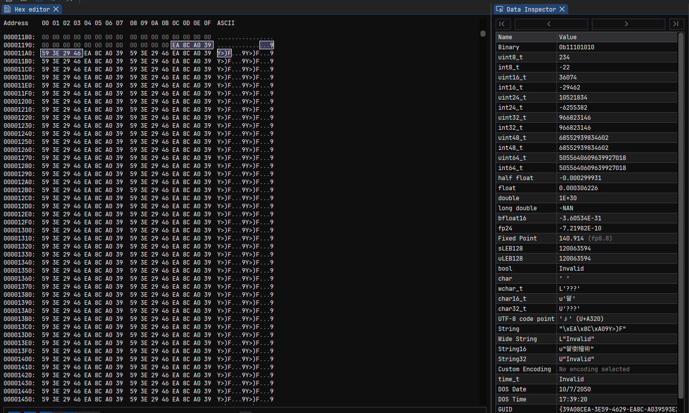
ImHex helpfully shows us a list of potential interpretations over on the right in the “Data Inspector”; the interesting options for us are “float” and “double”; the “float” value interprets the first four bytes as a 32-bit little-endian floating point value while the “double value” interprets all eight bytes as a 64-bit little-endian floating point value: 1.0x10^30. That’s a nice round, if large, number, and a single repeated 64-bit value makes more sense than a pair of alternating repeated 32-bit values. At this point, we suspect we’ve found the offset of the data array, that it’s 64-bit “doubles”, and that 1e30 holds some special significance, at least for this grid.

Scrolling to the end of the file, we see a lot of the same “stuff”: lots of 0xEA8CA039593E2946, some other values in the middle. Highlight a few and see values like 181.85: a nice thickness in feet for the Utica? Ok, let’s test an assumption: the data array begins at offset 0x199C and lasts until the end of the file. Let’s grab our handy Python interpreter and try to load that data as a floating-point array, then poke it a bit, maybe blit it to a graphic and see if anything pops out.

import numpy as np
import matplotlib.pyplot as plt

# open in "binary mode" (don't fiddle with newlines - just the bytes ma'am)
with open('UTICA_ISOPACH.GRD', 'rb') as f:
    buf = f.read()

# build a NumPy array from our potential data array
grid = np.frombuffer(
  buf,
  dtype=np.dtype(float).newbyteorder('<'), # 64-bit "doubles", little-endian
  offset=0x119c # starting at our known offset
)

print(f'{grid.shape=}')
print(f'{grid.max()=}')
print(f'{grid.min()=}')
# a hunch: what's the mean if we ignore all the 1e30s?
print(f'{grid[grid != 1e30].mean()=}')

Give that a spin and:

grid.shape=(18792,)
grid.max()=np.float64(1e+30)
grid.min()=np.float64(-74.44292240134156)
grid[grid != 1e30].mean()=np.float64(137.96704690045632)

Ok, promising. We can’t plot it yet because we’ve got a huge 1-dimensional array; we know the real data must be 2-dimensional. There are surprisingly few candidate sizes:

for rows in range(1, len(grid) // 2):
    if len(grid) % rows != 0:
        continue
    print(f'Candidate size: {rows} x {len(grid) // rows}')

That gives us a list which I’ll cut down to only candidates with plausible aspect ratios (it’s likely our region is closer to a square than to a long strip):

Candidate size: 108 x 174
Candidate size: 116 x 162
Candidate size: 162 x 116
Candidate size: 174 x 108

Let’s try reshaping and plotting:

fig, axs = plt.subplots(2, 2)
for ax, rows in zip(axs.flatten(), (108, 116, 162, 174)):
    cols = len(grid) // rows
    grid2d = grid.reshape((rows, cols))
    ax.set_title(f'{rows} x {cols}')
    ax.imshow(grid2d)
plt.show()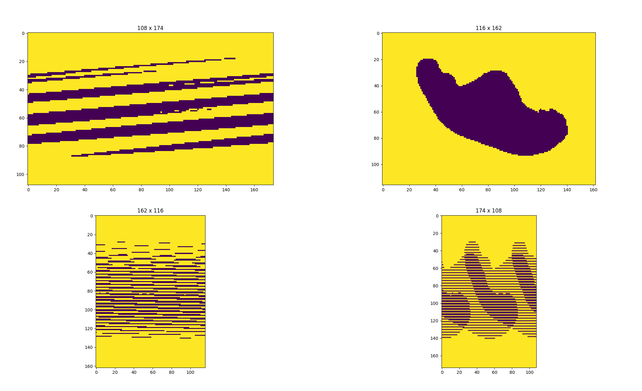

A ringing endorsement for 116x162! (I do like the look of 174x108, though - I’d probably put that on my wall! My wife would kill me, but I might.)

In what will become a pattern, let’s take this new knowledge and look for those values in the header of the file. Somewhere in there, we expect to find, most likely, 116 and 162 as integers. They’ll probably be 32-bit integers, because that was the “native” integer size at the time and because that’d support up to 4-odd billion rows. 16-bit integers would be possible, but limit the application to no more than 65,536 rows or columns. 64-bit integers would be possible too, I suppose. It’s also possible Petra only stores the row count and total cell count, or the column count and total cell count; or maybe it stores the size in bytes rather than values (so multiply by eight; well, no, there’d be a “stride” to store to make that work efficiently…) - enough blathering! Reverse engineering is an empirical art; let’s look for what we expect to find. I use ImHex’s search function to seek through the entire file for a uint32_t (that is, an unsigned i.e. non-negative 32-bit integer) with value 116, and behold:

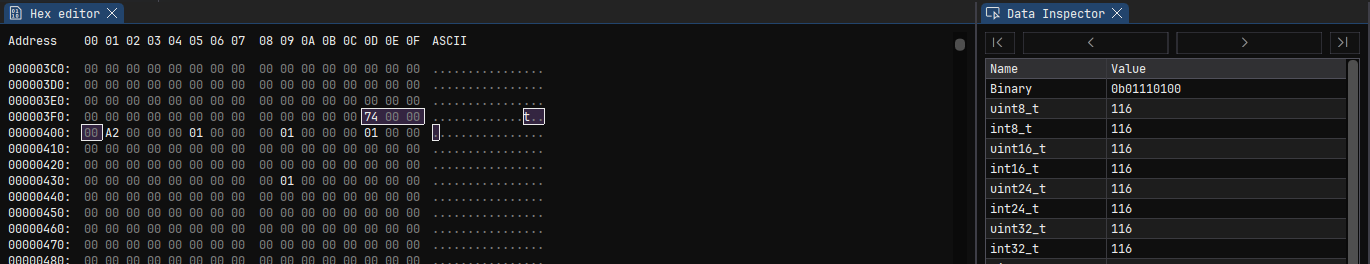
There it is! And what’s this 0xA2000000 right on its heels? Why, it’s our old friend 162! Now we know the offset of the size in one dimension (0x3FD) and the size in the other (0x401). I’m careful not to say “rows” and “columns” here as we don’t know which is which yet for sure. At this point in the real story, I had a known grid to compare. I transposed, mirrored, and so forth until I knew which one was rows and which one was columns, and I knew which way was east and which way was south.

Now, what about those 1e30s? As I explored the data files I was also searching any Petra documentation I could get my hands on. Here’s something interesting, albeit not from the grid module’s documentation: “When a bound cell is left blank, the associated range value is set to 1E30.” Let’s try treating that as a null/missing sentinel value. (I’ll also add the corrected row order to match the default orientation of imshow plots with the correct north/south direction.)

grid = grid.copy()
grid[grid == 1e30] = np.nan
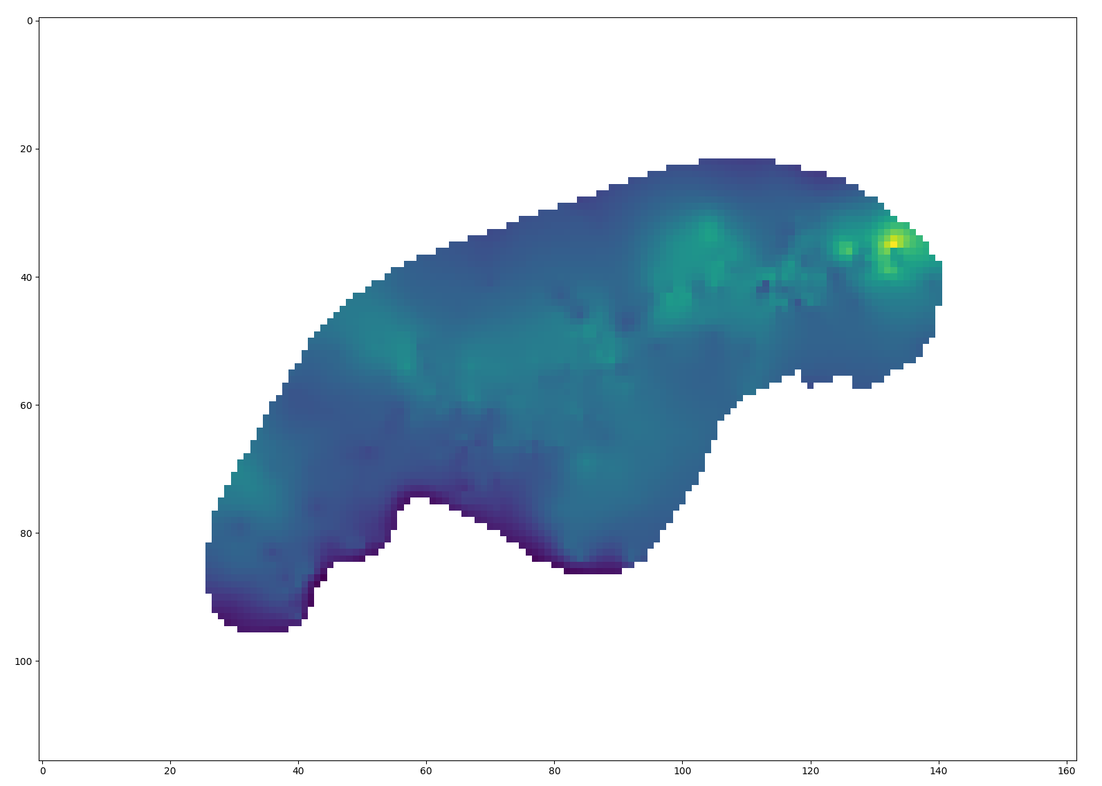
grid2d = np.flip(grid.reshape((116, 162)), axis=0)
plt.imshow(grid2d)
plt.show()

Hey, that looks like a plausible isopach!

There are still some issues: we don’t know the mapping between x and y grid indices and real-world units. We don’t know what most of the “stuff” in the header is. If we try the same logic on, for instance, some of the structure maps in the Utica data set, we’ll find that the number of grid entries doesn’t make sense at all. Tragically, though, I’ve already overshot my word count budget for this article by a considerable margin; mercifully, I’m going to hit the highlights on my way out the door rather than continue in all the gory detail.

Much of the remaining work went in the way you might now be equipped to imagine: look for interesting values in the header, form a hypothesis, test on the data. Rinse and repeat. In this fashion I worked out that the header stored a grid label, a total cell count, minimum and maximum values for the real-world dimensions of the x and y axes, and grid cell sizes in those dimensions. One with access to Petra, or an ancient demo thereof, and a Delphi decompiler might have been able to solve many of the remaining mysteries by taking the application apart and tracing the logic of key routines (say, the function that writes .grd files to disk); such a one might even find a helpful sequence of calls to Delphi’s equivalent of printf revealing offsets of key data items, perhaps like:

0043591D        lea         eax,[ebp-2A4]
00435923        mov         dword ptr [ebp-2C4],eax
00435929        mov         byte ptr [ebp-2C0],3
00435930        lea         edx,[ebp-2CC]
00435936        mov         ecx,1
0043593B        mov         eax,43880C;'XINC=%f YINC=%f'
00435940        call        Format

Luckily for me, much was instead revealed to me in a dream.

There was also the matter of “triangulated grids”: it turned out that when faults were present, Petra did not calculate regular rectangular grids but rather meshes of triangles very familiar to anyone with an interest in 3D graphics. This was discovered when a basic sanity check (rows x cols = number of values in grid) failed on an example grid. This too took some iterative investigation, but in the end I worked out that these were stored as a three-dimensional array: a sequence of triangles, with each triangle having three vertices and each vertex having x, y, and z coordinates. A wasteful representation, albeit one which makes rendering easy. (If you squint, you can see the tiny “gap” which caused the Utica structure map to need triangulation.)

The final product of all of this investigation was a big wooly loader script and a set of alarmingly haphazard notes; I turned the first into a Rust library and the second languished in my personal Vimwiki. I also created a simple set of Python bindings to the Rust library; you can install this from PyPI and “it just works” - at least for the subset of Petra grids I was able reverse engineer!

If you’ve made it this far, thank you - I wanted to convey something of the real texture of the activity, even at the expense of boring the majority of the audience. “A day in the life”, right? Reverse engineering isn’t a skill set I use every day, but it’s come in handy more than one might guess. Petra grids are a great example that I’ve used to support client projects and had the opportunity to release as an open-source toolkit, but I’ve also taken a crack at SMT Kingdom grids, debugged broken spatial database implementations, hot-patched Spotfire to let me circumvent UI limitations, and more I probably shouldn’t talk about too much! There’s no magic to it, just a methodical application of knowledge and experimentation to build understanding.